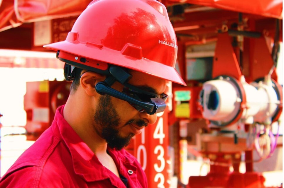
Halliburton reservoir testing and analysis illuminates the subsurface, giving operators a clear view into the reservoir.
talk to an expertTesting is vital to reservoir understanding and requires testing tools and systems that provide dynamic control and analysis in real time. Halliburton’s extended well testing portfolio gathers critical data operators need most, from downhole temperature data to reservoir samples to subsea safety systems. This data provides a full view into reservoir permeability, skin, initial pressure, and more, enabling better decision-making.
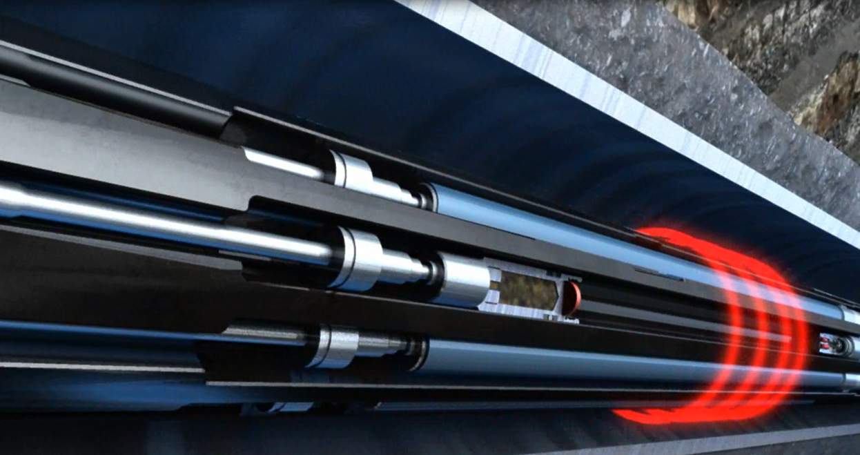
A comprehensive, fully acoustic downhole well testing system
Learn More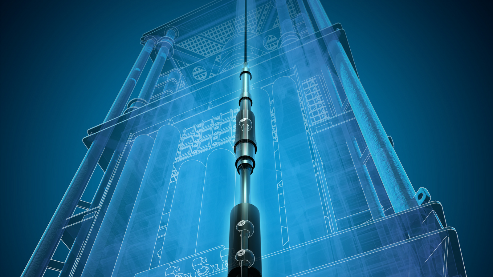
Safe well access for landing strings
Learn more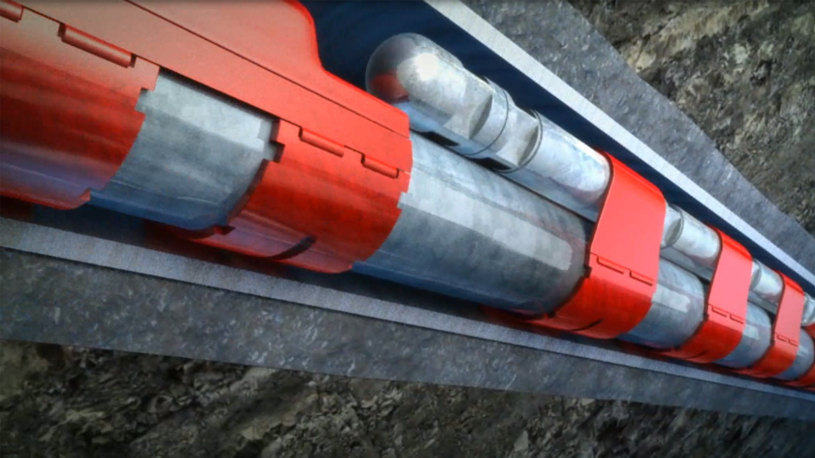
Real-time data, decisions, and control
learn more
Surface well testing equipment and solutions compile full and reliable data, enabling better reservoir evaluations and appraisals
Learn more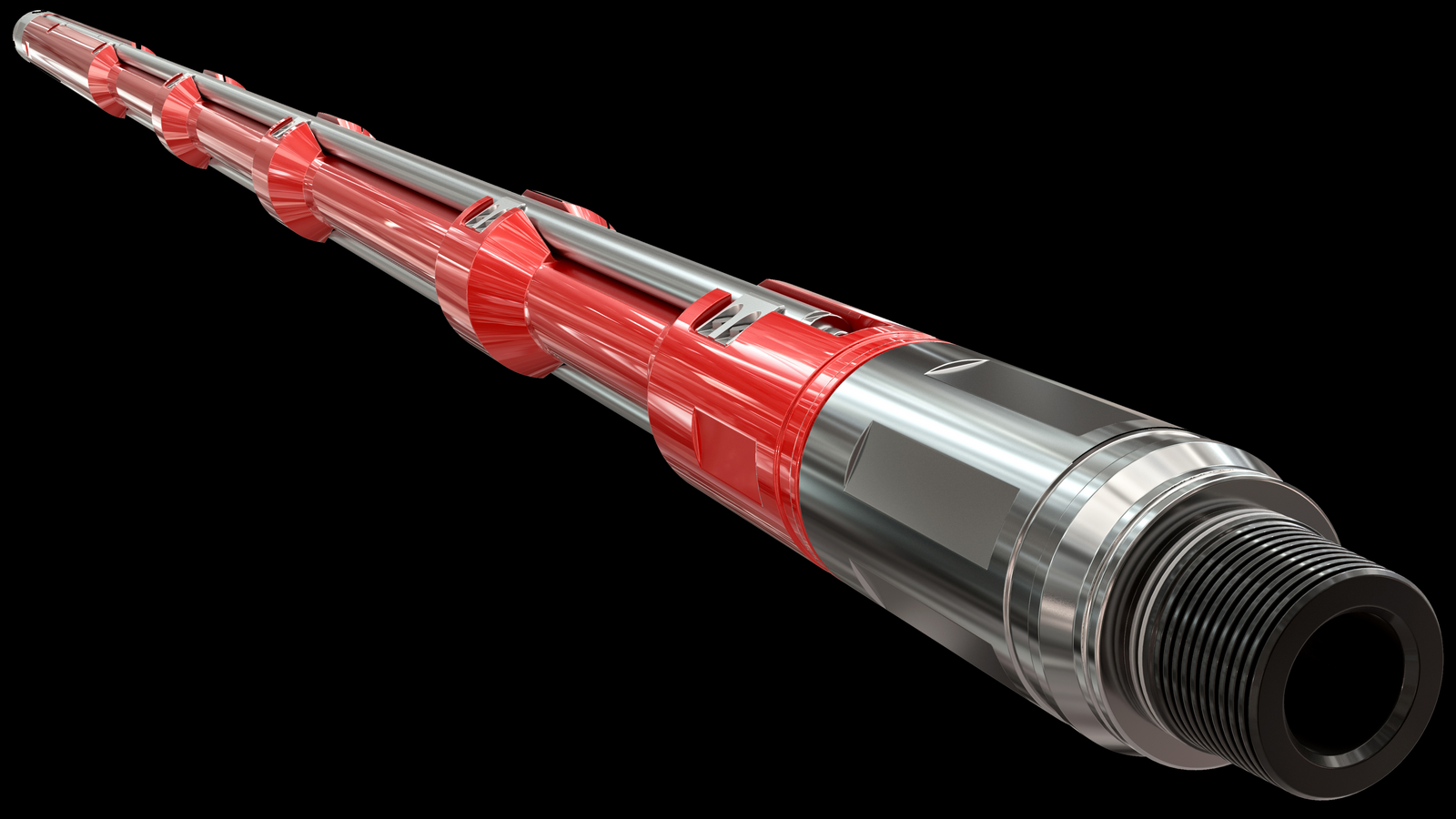
On demand real-time bottomhole positioning without intervention
LEARN MORE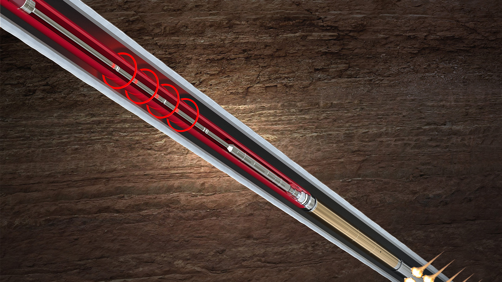
Safe and reliable wireless initiation of tubing-conveyed perforating
Learn More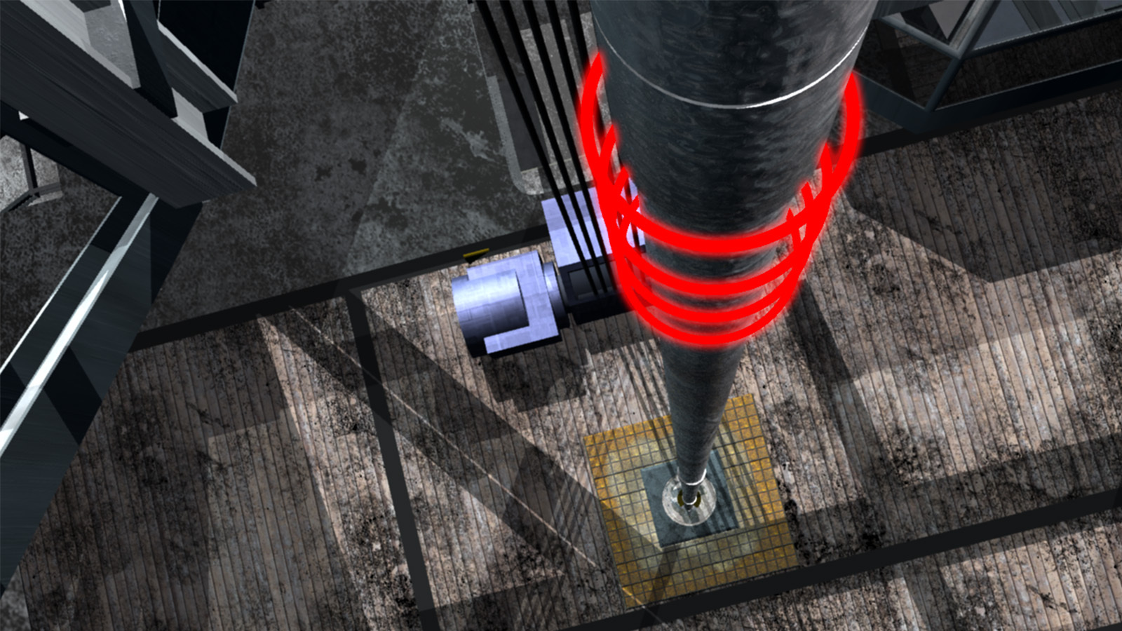
Real-time well testing solutions for measuring and analyzing well-test data.
Explore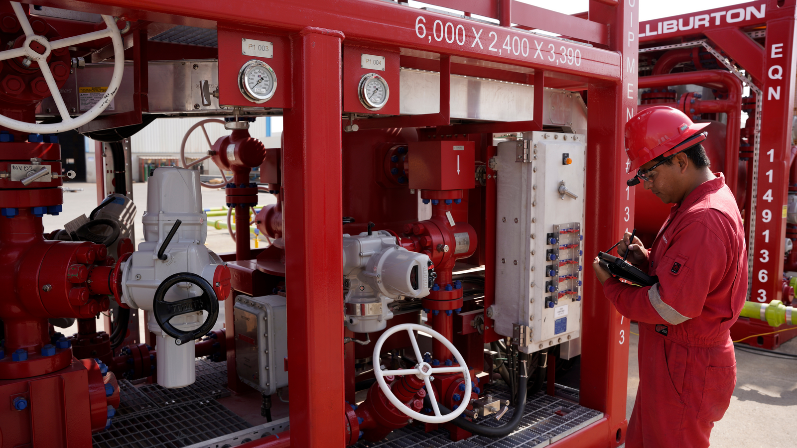
Halliburton surface well testing (SWT) tools and solutions compile full and reliable data, enabling better reservoir evaluations and appraisals.
Explore
Deepwater safety solutions for exploration, appraisal, completion, and intervention.
Explore